%20(1)-1.png?width=575&name=Data%20(2)%20(1)-1.png)
Emissions Reduction Potential: EPA’s Site-Level Emissions Estimates Compared to Measurements During Gas Mapping LiDAR Field Operations
The goal of an oil and gas company’s methane leak detection and repair (LDAR) program is to effectively and efficiently detect and reduce fugitive methane emissions in their infrastructure. Historically, LDAR programs have used optical gas imaging (OGI) cameras as the workhorses for detecting methane emissions. More recently, advanced detection technologies, including Bridger Photonics’ (‘Bridger’) Gas Mapping LiDAR (GML), have emerged with the hope of providing more effective methods for accomplishing the same goal.
As part of its recently proposed New Source Performance Standards (NSPS) methane rule¹, the U.S. Environmental Protection Agency (EPA) provided site-level emissions estimates to determine the emissions reduction potential of their standard (OGI-based) LDAR program (‘Standard Program’). So, here at Bridger, we jumped on the opportunity to compare these EPA estimates to the emissions that we detect during operations in the field with GML. This blog is devoted to putting some important context behind our finding that the potential emissions reduction from GML’s measurements far exceeds the reduction potential based on the assumed emissions from EPA’s Standard Program.
EPA’s Standard LDAR Program: Estimated Emissions Detection and Potential Reduction
OGI cameras have been the mainstay for detecting methane leaks in LDAR programs for many years. OGI cameras utilize the absorption of thermal infrared radiation by methane gas to detect and image leaks. LDAR programs using OGI typically involve visiting oil and gas facilities with ground crews and scanning equipment with handheld OGI cameras in search of leaks.
In EPA’s recently proposed NSPS methane rule, quarterly OGI scans of regulated equipment were proposed, with an estimated 80% emission reduction at this scan frequency. Digging deeper, the Regulatory Impact Analysis (RIA)² for the Proposed Rule includes the EPA’s associated average baseline emissions estimates for different regulatory ‘bins’, or emission categories (Table 2-4 in the RIA). We used this information to calculate the weighted average of emissions for each category of site. The largest of these weighted average estimates among the scenarios considered by EPA in the RIA was 9.91 tons per year (tpy). So, we consider a 10 tpy site to be a conservative (i.e. high) estimate of the EPA’s assumed average emissions at a typical site. Using this value for the average emission per site, the EPA would estimate the potential to reduce methane emissions by 8 tpy per site (i.e. 80% reduction¹ from 10 tpy—see Figure 1 for EPA’s emission reduction vs. scan frequency estimates) using this Standard Program.
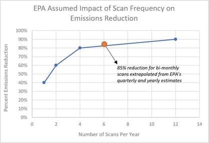
Figure 1. EPA's assumed impact on emissions reduction based on the number of scans per year (scan frequency). Plot created by Bridger Photonics using EPA data.¹
10 tpy×80% emission reduction factor
= 8 tpy potential emissions reduction per site
using EPA' s Standard Program (OGI scans)
Real-World Emissions Detection and Potential Reduction with Bridger’s Gas Mapping LiDAR Alternative Program
Bridger Photonics’ GML program uses LiDAR technology deployed on aircraft to detect, image, and quantify emission sources. Learn more about Gas Mapping LiDAR here.
As a substitute to quarterly OGI scans, the EPA’s proposed alternative program (‘Alt Program’) comprises bi-monthly aerial scans (six per year) using an alternative technology (e.g. with GML) plus one annual OGI scan. To calculate the emission reduction potential for the bi-monthly GML scans, we used actual Bridger Photonics data of emissions from over 12,000 production facilities in five major North American basins. To determine average emissions per site, we took the total number of emissions and divided it by the total number of sites (including sites with no detected emissions), which yielded an average annual emissions rate of 8.3 kg/hr, or approximately 80 tpy, per site. We then multiplied this by 52% to exclude the 48% Normal Operating Process Emissions, or NOPEs, that we detect (based on client-reported data). Note that this client-reported identification of NOPEs versus fugitive emissions is only an estimation, and understanding these relative proportions is an active area of Bridger research and client discussions. Next in our calculations, we multiply the result by an 85% reduction factor to account for our bi-monthly scan frequency (based on EPA’s estimated emission reduction factor for a given scan frequency shown in Figure 1; 85% reduction was extrapolated between the EPA’s 80% reduction for quarterly scans and 90% reduction for monthly scans). These calculations yield approximately 35 tpy of potential emissions reduction at a site.
If we then include the EPA’s proposed additional single annual OGI scan for the Alt Program, assuming the EPA’s approximate average of 10 tpy site (as described above, rounding conservatively up based on the highest weighted average of emissions categories from EPA’s RIA for the Proposed Rule), and the 40% EPA reduction estimate for an annual scan, we add 4 tpy emissions reduction potential for this OGI scan. This additional scan, combined with the 35 tpy emission reduction potential we calculated above for the bi-monthly GML scans, results in a total of 39 tpy. This straight addition of the contributions assumes that the OGI and GML scans are independent (i.e. if OGI catches leaks, it doesn’t affect the leaks caught by GML, and vice versa). While this assumption is not exactly true, it is likely reasonable because (a) the OGI scan can be spaced in time well away from the GML scans, and (b) third party evidence³ and anecdotal client feedback indicate that OGI and GML scans are largely complementary to one another; OGI generally detects smaller leaks and GML detects larger leaks.
So, for the EPA’s Alt Program using GML for bi-monthly scans plus one annual OGI scan, an estimated 39 tons of methane per year, per site, would be potentially reduced and available for recapture. This result excludes NOPEs, is based on the EPA’s assumptions described above, and applied to the actual average emission rate for over 12,000 sites measured during operations in the field using GML.
80 tpy (GML measured) × 52% NOPE exclusion × 85% emission reduction factor
+ 10 tpy (EPA OGI estimate) × 40% emission reduction factor
=35 tpy + 4 tpy
= 39 tpy potential emissions reduction per site
using EPA's Alternative Program (GML scans + single OGI scan)
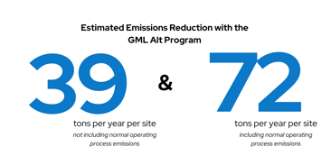
Using the proposed Alt Program with GML, we recommend that the EPA does not require operators to visit identified NOPEs with ground crews until the next annual OGI scan unless the emission rate exceeds that permitted for the equipment in question. Nevertheless, our clients typically appreciate our identification of NOPEs because it provides them with more opportunities (e.g. equipment retrofits and upgrades) to reduce emissions. If we include NOPEs in our calculations for potential emissions reduction using GML, an 80 tpy site with an 85% assumed reduction rate as described above for bi-monthly scans, we estimate 68 tpy of methane could be reduced—which, combined with an additional 4 tpy for the single OGI scan, results in a total of 72 tpy of emission reduction potential per site.
How Do Gas Mapping LiDAR’s Emissions Reduction Estimates Compare to EPA Estimates?
From the above analysis, we estimate the GML Alt Program to have nearly five times the emissions reduction potential per site compared to the EPA’s Standard Program using OGI (39 tpy of methane versus 8 tpy). While this is a powerful result for the oil and gas community, especially considering the Alt Program with GML costs less, the results need context for a proper assessment.
First, the EPA’s estimated emissions are based on emissions factors, not actual measured emissions detected using OGI. Emission factors are emissions estimates assumed to occur from typical equipment leaks found on production facilities. But, there is considerable uncertainty regarding whether these emissions factors are accurate representations of actual emissions.⁴ The GML calculation, on the other hand, uses actual measured emissions from sites where GML has been used, rather than modeled or estimated emissions. Additionally, GML detects all emissions from the production facility, not just the equipment included in an LDAR program. Finally, the EPA itself emphasizes in the Proposed Rule that its emissions estimate “calculations are based on the expected reductions from ‘typical’ component equipment leaks that occur with well-maintained sites”¹ and acknowledges “malfunctions related to equipment components can cause large emission events”¹ that may result in “significantly higher”¹ estimates. So, this is not an apples-to-apples comparison between the EPA’s Standard Program using OGI and the Alt Program using GML.
Nevertheless, the emissions reduction potential for the Alt Program with GML is based on actual measured data and conservative assumptions. This means Bridger’s GML provides oil and gas operators with the opportunity to remove, on average and across North American basins, a minimum of 39 tpy of methane emissions per site from their annual emissions inventories. If retrofitting NOPEs is included in an operator’s sustainability plan, then this moves up to 72 tpy per site.
Good for the Environment and for Business
Emissions factors and the EPA estimates aside, there is growing third-party evidence indicating that GML does catch more emissions than OGI. Recent peer-reviewed research⁵ indicates that GML detects far greater total emissions from an average oil and gas production site than with traditional OGI scans. In two of our previous blog posts we describe the highlights of these studies: Key Takeaways from EERL's “Where the Methane Is” Study and Key Takeaways from EERL’s “Blinded Evaluation of Airborne Methane Source Detection". Moreover, while GML detected greater emissions, these emissions came from far fewer leak sources (i.e. fewer repairs for operators). So, this represents a rare win-win for the environment and the industry.
Taking this one step further, when emissions are detected and repaired, this presents an opportunity to recapture natural gas for revenue production. In the next blogs in this series, we’ll walk through the potential cost savings of using GML scans, and the even greater savings when gas is recaptured and converted to revenue.