
A new peer-reviewed publication by emissions researchers at Bridger Photonics has been published in Environmental Science & Technology. This study fills in a large portion of the distribution of emission rates observed from Permian Basin oil and gas production infrastructure that had not previously been directly measured at scale.
This study used Bridger Photonics’ Gas Mapping LiDAR™ (GML) technology to aerially scan wells and other production infrastructure at 7,474 facilities in the Midland and Delaware sub-basins, detecting methane emission rates down to roughly 2 kg/hr at 90% probability of detection (PoD).
The GML data were combined with data from previous large-scale, less sensitive measurement campaigns conducted by Carbon Mapper (CM) (reported in Cusworth et al., 2021 and 2022—see below for full references) which used aerially deployed high-altitude solar infrared (IR) imaging technology to detect emissions in the same area. Comparison of the two datasets show that the detection sensitivity of the CM campaigns was 280 kg/hr at 50% PoD for “facility-sized” emission sources (150 m diameter), which may be comprised of emissions from multiple assets, and 320 kg/hr at 50% PoD for “equipment-sized” emission sources (∼2 m diameter).
The CM sensitivity limitations mean that emissions smaller than these thresholds went undetected more often than not in those campaigns. The new data from GML, at a significantly better detection sensitivity, then allows insight into a large segment of the methane emission rate distribution for the oil and gas production sector that until now had been undermeasured in the scientific literature: the segment from 3 kg/hr up to roughly 300 kg/hr.
Here are the key takeaways from the study:
Takeaway 1: Mid-range emission rates (3 - 300 kg/hr) are much more common than previously reported.
GML scanned a similar set of infrastructure with a better detection sensitivity than CM, and many more emissions events were detected. Emissions were detected at 38.3% of facilities flown by GML, compared to 1.5% of facilities flown by CM. Most of the emissions found by GML were below the CM detection sensitivity, so these would have been mostly undetected during the CM campaigns.
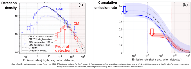
The very high prevalence of mid-range emission sources (3-300 kg/hr) can be seen in Fig. 1. This figure plots the density of detected emission sources across GML and CM campaigns after controlling for differences in spatial scale and number of overflights. Whereas CM’s PoD begins to diminish at emission rates below the full detection limit (FDL), where the PoD is roughly 100%, at 600 kg/hr (left edge of the shaded area in Fig. 1a), GML’s fully measured distribution continues down through emission rates as low as 3 kg/hr for equipment-sized sources (dotted vertical blue line in Fig. 1a). Comparing detection densities shows a wide gap between CM and GML detection rates. For example, at 100 kg/hr, GML detected 14 times more facility-sized emission sources (black vertical line in Fig. 1a) than CM detected at this emission rate. The difference may be even larger for equipment-sized emission sources.
The cumulative emission rate corresponding to these measurements is shown in Fig. 1b. The impact of detecting many more sources below CM’s full detection limit is shown by the GML cumulative emission rate (blue line) extending well above the CM cumulative emission rate (red line). Despite their smaller individual emission rates, mid-range (and smaller) emission sources below the CM FDL are so common that they contribute a majority of the total cumulative emission rate. This can be seen by comparing the total cumulative emission rate measured by CM (red arrow) to the total measured by the GML (blue arrow).
Why It Matters:
Emissions below the CM FDL (less than 600 kg/hr) have a significant impact on the cumulative emission distribution, and their partial absence leads to significant underestimation of emission rate totals. Understanding the true prevalence of emission sources from large to small is essential to inform emissions measurement campaigns and build efficient and effective mitigation strategies.
Takeaway 2: The spatial scale to which emission sources are resolved affects the measured emission rates and their corresponding distribution.
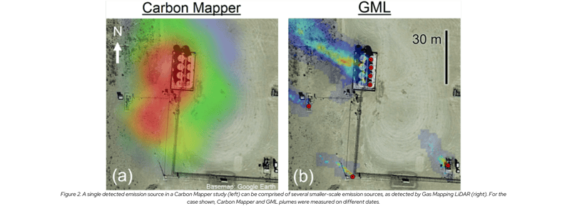
Whereas equipment-resolved source detection yields pinpoint location data that is essential for emissions screening and identification, not all emission quantification campaigns resolve sources to this level. For instance, in the CM studies, the aim was to cover a very large geographic area with multiple overflights at high flight altitudes (4.5 and 8 km above ground level) so the entire area could be covered in a short time frame. Due to constraints from image resolution and strategies to track emission source intermittency, emission sources were reported using a 150-meter diameter aggregation area. GML sensors are flown much closer to the ground (200 m) and emission point source locations are resolved to a precision of 2 m, enabling equipment-sized identification of emission sources. An example is shown in Fig. 2, where a facility-resolved methane plume measured by CM may be comprised of one or more underlying equipment sources that are aggregated into a single plume (Fig. 2a), whereas emissions from individual equipment sources are identified by GML (Fig. 2b).
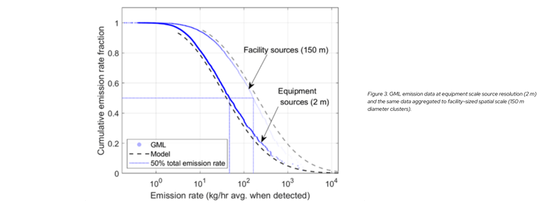
A pitfall of reporting emission rates at the facility-aggregated level is that emission rate distributions show a higher density of large emission rate sources from summing the contributions of possibly multiple constituent equipment-level sources. An example of this is shown in Fig. 3. For the “facility source” trace, GML-measured equipment sources within 150 m of one another have been added together to count as a unique emission source roughly representing a facility at the size of a typical well pad (150 m). For the “equipment source” trace, emission rates were kept at the 2 m source resolution measured originally. Aggregation to facility-sized sources shifts and reshapes the distribution to larger emission rates, which impacts the apparent sensitivity required to detect a given fraction of total emissions. To detect 50% of the total emission rate in this distribution (horizontal dotted line), a sensitivity of 50 kg/hr is required for equipment-sized sources. This increases to 160 kg/hr for facility-sized sources.
Why It Matters:
For facility-resolved emission sources, a single detected “emission” may actually be an aggregate of several equipment-sized emissions on the same site. This is problematic because it inflates the apparent effectiveness of poorer detection sensitivity if emission sources are in fact detected on the asset level.
In addition, whereas a single emitter below the detection sensitivity may be missed, multiple emitters combined across a site could exceed the detection sensitivity. If this were the case, then the observed probability of detection for facility emission rates would then depend on spatial factors influencing whether a cluster of emitters is detected (e.g. whether emitters tend to be close together or far apart on sites), meaning that sensitivity found for a facility emission rate distribution may not be the same as another distribution with different spatial characteristics per facility.
Takeaway 3: The detection sensitivity of a less sensitive methane emissions detection campaign can be verified using a more sensitive detection campaign.
With a detection sensitivity of 2 kg/hr at 90% PoD for equipment-sized sources in the environmental conditions present during the scans, GML was used to evaluate the practical detection sensitivity of the CM campaigns. This comparison quantified the CM campaign detection sensitivity at 280 kg/h for facility-sized sources, as indicated by the small green vertical bar in Fig. 1a, which shows where the CM to GML ratio in detection density is 50%. This value provides a quantitative assessment of CM’s effective field-assessed detection sensitivity, which had been suggested in previous studies but not rigorously defined (Chen et al. 2022, Yu et al. 2022). Knowing the detection sensitivity is essential to understand how much of the emission rate distribution was missed in a given measurement campaign.
Why It Matters:
Third-party analysis with a more sensitive detection technology can provide a critical check on the claimed specifications of a technology. Controlled release testing is the gold standard for sensitivity characterization, but results depend on a range of environmental and flight parameters. Whereas these parameters (including wind speed, flight altitude, ground cover, etc.) can be accounted for in controlled release as described in Conrad et al. (2023), evaluation of “in the field” sensitivity by comparing to a set of more sensitive measurements can provide valuable insight into a campaign’s performance.
Thank you to the research team at Bridger Photonics, the peer-reviewers for the study, and the team at Environmental Science & Technology.
Read the full study linked here.
References:
Cusworth, D. H.; Duren, R. M.; Thorpe, A. K.; Olson-Duvall, W.; Heckler, J.; Chapman, J. W.; Eastwood, M. L.; Helmlinger, M. C.; Green, R. O.; Asner, G. P.; Dennison, P. E.; Miller, C. E. Intermittency of Large Methane Emitters in the Permian Basin. Environmental Science and Technology Letters 2021, 8, 567–573.
Cusworth, D. H.; Thorpe, A. K.; Ayasse, A. K.; Stepp, D.; Heckler, J.; Asner, G. P.; Miller, C. E.; Yadav, V.; Chapman, J. W.; Eastwood, M. L.; Green, R. O.; Hmiel, B.; Lyon, D. R.; Duren, R. M. Strong methane point sources contribute a disproportionate fraction of total emissions across multiple basins in the United States. Proceedings of the National Academy of Sciences 2022, 119, e2202338119.
Chen, Y.; Sherwin, E. D.; Berman, E. S. F.; Jones, B. B.; Gordon, M. P.; Wetherley, E. B.; Kort, E. A.; Brandt, A. R. Quantifying regional methane emissions in the New Mexico Permian Basin with a comprehensive aerial survey. Environmental Science and Technology 2022, 56, 4317-23.
Yu, J; Hmiel, B.; Lyon D. R.; Warren, J.; Cusworth, D. H.; Duren, R. M.; Chen, Y.; Murphy, E. C.; Brandt, A. R. Methane Emissions from Natural Gas Gathering Pipelines in the Permian Basin. Environmental Science and Technology Letters 2022, 9, 969−974.
Conrad, B. M.; Tyner, D. R.; Johnson, M. R. Robust probabilities of detection and quantification uncertainty for aerial methane detection: Examples for three airborne technologies. Remote Sensing of Environment 2023, 288, 113499.